What do you mean you don't do indexing?

When I talk to people about Parseable’s architecture, the conversation usually gets to the same place: how is this different from a traditional time series database, and where is the metric index? If we don’t keep an inverted index for every label, how does a query find the right samples?

We do use selective indexes and pruning metadata. We don’t maintain a TSDB-style lookup from every metric label value to a list of series.

For PromQL queries over Parquet, time partitions and manifests narrow the files. Parquet statistics and page indexes narrow what we read inside them. A Bloom filter can rule out row groups that don’t contain the metric name. DataFusion pushes filters into the scan and verifies the rows that remain. Let’s follow one query through that path.

Take a query you might put on a dashboard:

rate(http_requests_total{service="checkout"}[5m])

It asks for one metric, one label value, and five minutes of history for each evaluation point. Imagine that the stream also contains thousands of other metrics and millions of resource IDs. We need to find the matching samples without turning every refresh into a tour of object storage.

In a series-first TSDB, an inverted index can map a label value to the series IDs that contain it. That’s useful. It also means maintaining those lists as new label values and series appear. We store metric samples and labels as columns in Parquet instead. A new resource ID is another column value. It doesn’t need an entry in a separate label-to-series lookup structure. The price is that a query must scan the data that survives pruning. So which files can it rule out before opening them?

Start at the writer, not the query

A Parquet file isn’t one indivisible blob. It contains row groups. Each group has a chunk for each column, and those chunks are divided into pages. A reader can skip a whole row group, a few pages, or columns it doesn’t need. But those options are only useful if the writer gives the reader enough information.

For OpenTelemetry metric streams, our conversion path buffers records for a row group and sorts them by metric name ascending, then by ingestion time descending. Prometheus remote write is normalized into this metrics path, so it gets the same layout. The writer records the sort order in Parquet metadata and writes a Bloom filter for the metric-name column.

So, if a page contains a mix of nearly every metric name, its minimum and maximum names span most of the stream. The page index, which records page-level statistics, can’t rule out much. Put nearby names together, and a page can have a much tighter range. A direct metric selector like the one above then has a better chance of skipping pages.

Why put the Bloom filter on the metric name rather than every label? A direct selector pins the name, so we can test the same column for many PromQL queries. Building filters for every pod, service, or resource attribute would cost space and write time whether or not anyone queried them. This is a targeted choice in the metric writer, not a switch we turn on for all telemetry.

Two clocks narrow the first read

Each sample has its own timestamp. We also partition stored data by ingestion time. They answer different questions. The sample time says whether a point belongs in the result. The ingestion time says where we should look for it.

The PromQL bridge computes exact sample-time bounds, including the history a range function needs before the visible start of the chart. It also adds bounds on the ingestion-time partitions so the storage layer can narrow the search. Those partition bounds are rounded to minute buckets, with roughly a minute of room after the requested end for ingestion delay.

That bound can hide very late data. If an old sample arrives hours after its own timestamp, a historical query with roughly a minute of ingestion slack may never look in the partition where it landed. If you backfill old samples, this is a real query behavior to account for, not just a performance trick.

Once the time window is known, the snapshot tells us which manifests to read. It lists their paths and time ranges. Each manifest lists Parquet files and file-level column statistics collected when those files are written to object storage. If the known min/max for the metric-name column rules out http_requests_total, we can leave that file unopened. The check is conservative. If statistics are missing, types don’t line up, or the predicate is too complex, we keep the file.

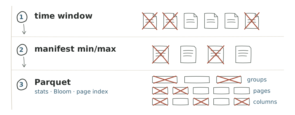
Even deciding what to skip takes work. The snapshot path fetches manifests concurrently and checks file statistics in parallel. Wide streams can leave hundreds of column descriptors on each rejected file entry, so the code even spreads their cleanup across threads. The query session also uses a 2 MiB Parquet footer-read hint to avoid a second object-store request for wide footers. None of that reads a sample, but it still takes time.

The gap that min/max leaves open

Suppose a row group contains api_errors_total and queue_depth. Alphabetically, http_requests_total falls between them. The min/max range says “maybe,” even though the name is absent. Sorting helps page ranges, but it doesn’t make a range into a membership test.

A Bloom filter hashes each value into a few positions in a compact bit array. If one of those positions is unset when we look for a value, that value is absent. If all are set, it may be present and the reader still checks the data.

That is the check we need here. Parquet stores a Bloom filter for the metric-name column in each row group where the writer enabled it. The split-block variant hashes a name into one 256-bit block and checks eight bit positions. An absent name lets the reader skip the whole row group, even when min/max said “maybe.”

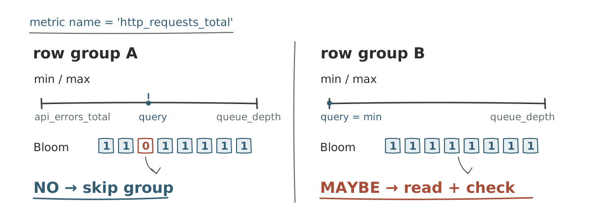
The filter does not return a row number, a series ID, or a list of matching files. It answers one membership question for one row group. Row-group statistics may already have rejected some groups before the Bloom filter is read. A Bloom check only has a chance to help on the survivors.

The page index and Bloom filter cover different misses. If the name is present, the Bloom probe says “maybe,” and page statistics can still skip pages containing other names. If the name is absent but sits between the row group’s minimum and maximum, the Bloom filter can reject the whole group. Neither check makes the other redundant.

That skip isn’t free. Our writer gives Parquet an expected distinct-value count of 32,768 for the metric-name column. That is a sizing hint, not a measurement of each row group’s actual metric count or a promised false-positive rate. Filters take bytes to store, work to construct, and sometimes another metadata read. We don’t have a measured, universal speedup to quote here. I’d measure how many row groups Bloom rejects after statistics have had their turn.

The predicate has to reach Parquet

A Bloom filter sitting in a file does nothing if the query engine never presents it with a simple equality. For the running example, the PromQL bridge produces predicates with this shape. These are descriptions, not literal column names:

metric name = http_requests_total
service label = checkout
sample time within the requested range
ingestion time within the selected partitions

The bounds and selected columns vary by query. The direct metric-name equality is what lets the reader probe the Bloom filter. For a nonempty label equality such as service="checkout", the bridge can also emit a plain column comparison. Wrapping a label column in a function to handle missing values is harder for simple Parquet statistics to reason about. Empty-string and regex matchers need different handling because PromQL has missing-label semantics to preserve.

There is no dedicated Bloom filter on service in this path. If its min/max statistics exclude checkout, DataFusion can reject that file or row group. If not, it evaluates the label predicate on the rows it reads. A selective looking label filter is only as useful as the metadata and layout behind it.

Between those predicates and a Bloom probe sits one more optimizer pass. Our table provider installs the exact partition-time predicates in its initial Parquet scan. It marks metric and label filters inexact. They may help prune data, but the query still has to enforce them on surviving rows. DataFusion’s physical filter-pushdown optimizer can then attach a supported metric-name equality to the Parquet scan. Our query session enables Parquet pruning, filter pushdown, and page-index reads. DataFusion’s Bloom-on-read option is on by default.

At table-provider construction
  Parquet scan predicate    ingestion-time range
  Inexact metric filter    metric name = http_requests_total
  ↓
After physical filter pushdown
  Parquet scan predicate    ingestion-time range
                            + metric name = http_requests_total
  Surviving rows           metric filter still enforced

Stop at the table provider and the Bloom filter looks write-only. Follow the final physical scan and you find the equality that the Parquet reader can use. For a surviving file, DataFusion can check row-group statistics, then available Bloom filters, then page indexes, and finally decode the projected columns. Every stage has to leave the query correct even when it cannot rule anything out.

The rows we still have to read

A narrow query can still have a lot of work left. DataFusion reads the surviving Parquet column ranges, from object storage or a local hot tier when one is available. Our small-reads post explains why the number and size of object-store requests matter even after pruning.

A recent query can also include Arrow batches and Parquet files still in staging. Those records haven’t gone through the snapshot-backed object-store path yet. The physical plan combines them with persisted data. Older data can use a legacy listing path. The diagram shows the persisted path. Some queries take other paths.

After the scan, samples still need to become series. At ingestion we write a compact series fingerprint based on the metric name and flattened label pairs. It helps the read side group samples by series. It is not an inverted lookup from service=checkout to a file location. The query still projects the label columns it needs to return the series. PromQL then has to do the actual rate calculation or aggregation.

Some queries won’t get much from this layout. A regex over metric names isn’t the same as one equality. A long time window reaches more manifests and files. A topk over millions of resource IDs still has to consider the matching resources before it can pick the top twenty. A file without the metric-name Bloom filter falls back to statistics and normal filtering. “Our queries are fast because Bloom filters” would be as misleading as “we don’t index.”

Our 100-million-series write-up describes why keeping high-cardinality context is useful in the first place. This layout is one way to keep that context without maintaining an inverted metric-label index for every value. It doesn’t make broad analysis free. The product also has a separate Tantivy-based search index path. This post is about Parquet-backed PromQL metrics.

If I wanted to know whether a change to this path helped, I’d look at the counts along the way: manifests considered, files rejected by stats, row groups rejected by stats versus Bloom, pages and columns read, object-store requests and bytes, and time spent in series reconstruction. An end-to-end latency number alone can’t tell me which layer did the work.

So yes, there is indexing in this path, but it is selective. We use time bounds, file and Parquet statistics, page indexes, and a Bloom filter for metric names to rule out data that cannot match. We don’t keep an inverted list from every metric label value to its series IDs. Whatever survives is still a scan.