How PromQL works on columnar Parquet

Tell a database engineer that you want to evaluate PromQL over Parquet files in an S3 bucket and the first reaction is usually a pause. Sometimes a laugh. Sometimes a very reasonable “wait, what?” I get the reaction.

At Parseable, we do this anyway. Usually, Parquet and object storage are easy to explain for logs, traces, and wide events. Flatten the data, keep it compressed, skip irrelevant columns, and let object storage handle the boring durability problem. Metrics are less forgiving. PromQL is not a row filter with nicer syntax. It expects labeled time series, lookback windows, counters that can reset, instant vectors, range vectors, and clear rules for when two streams are allowed to merge.

So the question is not “can Parquet store metric samples?” Of course it can. The harder question is: can a query path read Parquet cheaply and still rebuild the exact time-series view PromQL needs before any math happens?

Use one dashboard panel as the running example. It asks for 5xx request rate by service over the last 24 hours, evaluated every 30 seconds:

sum by (service) (
  rate(http_requests_total{status="500"}[5m])
)

That query has a small visual output, but it is not small work. A 24-hour range at a 30-second step has 2,880 evaluation timestamps. The first timestamp still needs the five minutes before the chart starts, because rate(...[5m]) cannot be calculated from one point. If the scrape interval is 30 seconds, each rate window may need roughly 11 samples per matching series. If 50,000 series match the selector, the engine is now organizing tens of millions of samples before the service-level line can be drawn.

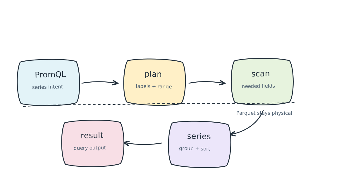
The storage layer should not make that worse. It should avoid reading every Kubernetes label, every resource attribute, and every metric in the file when the expression only needs a few fields. Parseable’s approach is to keep the storage format columnar, then do the PromQL-specific work at the boundary. The scan brings back the smallest useful slice of data. After that, the evaluator rebuilds series, range vectors, labels, and sample ordering carefully enough that the result still behaves like PromQL.

That boundary is where most of the engineering work lives.

The query budget

Here is the budget for the example query before any code runs:

Item	Value in this example	Why it matters
Visible range	24 hours	The chart window users asked for
Step	30 seconds	2,880 evaluation timestamps
Lookback window	5 minutes	Reads data before the visible start
Approximate samples per window	11 per series	5 minutes at 30-second scrape intervals, plus the boundary sample
Output grouping	service	The final result may have tens of services, not tens of thousands of pods
Series boundary	series_id	Needed so counter resets stay per stream

The output might be 20 or 50 lines in Grafana. The input is every sample for every matching series in the requested time range plus the lookback. That is why the planner has to be careful. It is trying to minimize bytes and columns without changing the semantic order of PromQL evaluation.

The semantic trap

Start with a query that looks harmless:

sum by (service) (
  rate(http_requests_total{status="500"}[5m])
)

If you come from SQL, the rough shape looks simple:

• Filter rows where status = '500'
• Group by service and compute a five-minute delta

That version is wrong in the one place where being wrong changes the graph.

PromQL does not first make one table of 500s and then compute a delta by service. It first finds the individual series that match the selector:

http_requests_total{service="checkout", status="500", pod="checkout-1a"}
http_requests_total{service="checkout", status="500", pod="checkout-2b"}
http_requests_total{service="payments", status="500", pod="payments-9c"}

rate(...) runs across the five-minute window for each one separately. Only after those per-series rates exist does sum by (service) collapse the values into a service-level answer.

Counter resets are the reason this ordering is not just a pedantic detail. If checkout-1a restarts while checkout-2b keeps serving traffic, mixing their samples before rate() can turn a normal restart into a fake drop and spike. The dashboard still draws a line. The line may even look plausible. It is just not the line you meant to ask for.

Until the range calculation is done, series identity has to remain separate.

Metric samples as wide rows

Metrics can arrive through OpenTelemetry or Prometheus Remote Write. By the time they are ready for storage, a sample has been normalized into a structured record and written to Parquet.

A stored row has the timestamp, metric name, value, labels, resource attributes, and enough metric metadata to make sense of the shape later. Keeping those fields queryable is the point. If status is a column, a matcher like {status="500"} has a chance to become real scan work instead of post-filtering after everything is loaded.

Two columnar features are doing the useful work here:

Predicate pushdown: A matcher like {status="500"} can be pushed toward the Parquet scan. Depending on file metadata and data distribution, the reader may skip unrelated files, row groups, or page ranges before decoding values.

Column projection: A query that never filters, groups, matches, or rewrites region should not carry region through the hot path.

For the running query, the first storage plan is not “read the metric table”. It is closer to this:

Field	Read?	Reason
timestamp	Yes	Build range windows and preserve sample order
value	Yes	Calculate rate()
metric_name	Yes	Select http_requests_total
status	Yes	Apply {status="500"}
service	Yes	Preserve the sum by (service) grouping key
series_id	Yes	Keep individual streams separate before rate()
pod	No, unless needed later	Already represented by series_id for boundary preservation
namespace, node, cluster, image	No	Not matched, grouped, joined, or emitted

That is the difference between carrying five or six hot columns and carrying the whole label universe. A Kubernetes metric can easily have 20, 40, or 100 dimensions once resource attributes and application labels are included. If every query has to load all of them just to be safe, the columnar layout is being wasted.

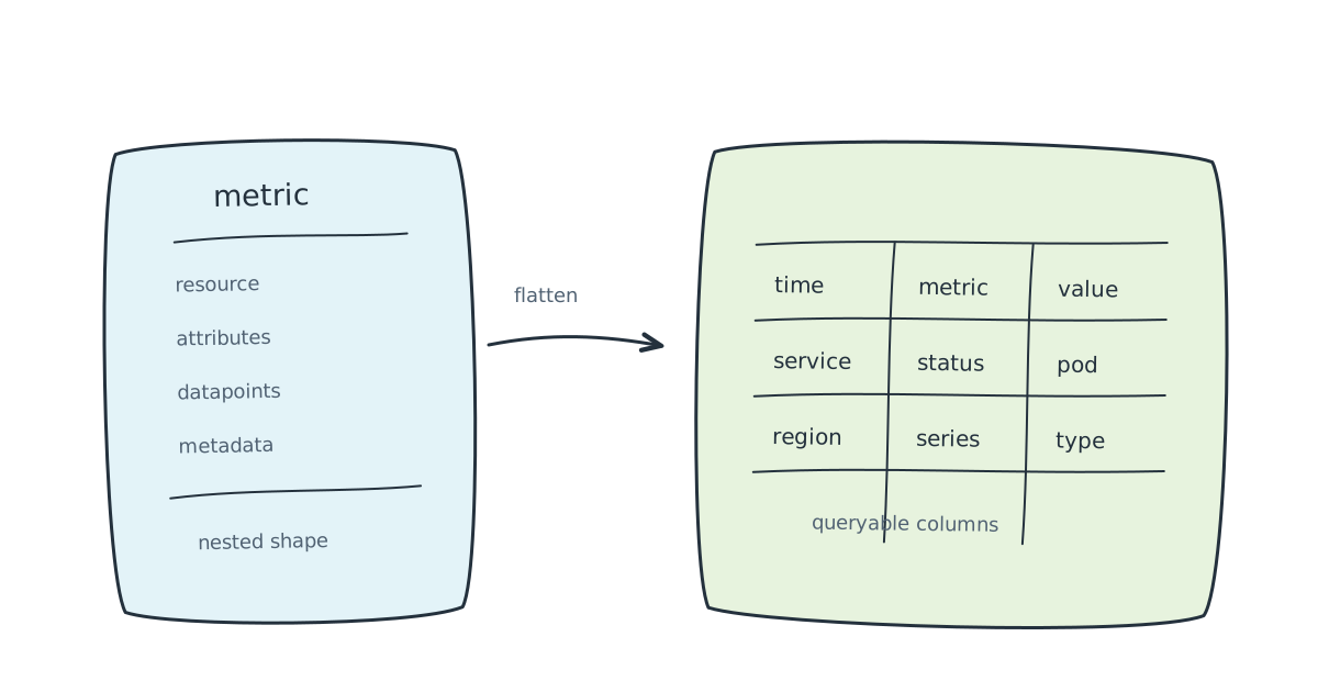
Kubernetes makes the problem less tidy. One workload can carry namespace, pod, container, deployment, node, cluster, instance, job, owner, image, build, plus OpenTelemetry resource attributes. Application code then adds its own labels. If every PromQL query has to read all of those string columns just to rediscover series boundaries, the system has lost most of the advantage of projection. It is still Parquet, but it is being used like an expensive wide scan.

The series identity problem

PromQL series identity is logically:

metric name + sorted(label key/value pairs)

A direct implementation can rebuild that identity while querying:

1. Read every possible label column.
2. Sort the label names for each sample.
3. Compare full label sets.
4. Group rows into series.

Easy to describe. Painful under high cardinality.

Parseable avoids doing that string-heavy reconstruction from scratch on every query. During ingestion, the metric path records a stable per-series identity that the query path can use later. I will call that compact identity series_id here. Treat the name as a concept for the post, not a public schema contract.

For the query above, the physical scan can stay close to this:

timestamp
value
series_id
status
service

timestamp orders samples. value is the raw counter. series_id preserves the physical stream. status satisfies the matcher. service survives because the outer aggregation needs it.

Notice what is not there: pod, namespace, node, cluster, image, and every other label attached to the metric but unused by this expression. The pod boundary is still safe because series_id carries it. The query only hydrates the labels it still needs to show or compute the result.

This changes the cost profile. The engine still has to process every matching series, but it does not have to materialize every label column for every sample. At high cardinality, that distinction matters. A stream identity can stay compact while the output labels stay precise.

There are two useful counts to keep separate:

Count	Example meaning	Why it can be very different
Matching series	Every pod, status, instance, and label combination for http_requests_total{status="500"}	This can be tens of thousands or more
Output series	One result per service after sum by (service)	This may be tens of services

The evaluator cannot jump directly to the second count. It must calculate rate() at the first count, then aggregate down. Columnar storage helps by making the scan narrower, not by skipping the PromQL order of operations.

PromQL is planner input

The query path cannot fire a Parquet scan and hope the PromQL evaluator sorts it out later. It has to inspect the PromQL AST before storage planning, because the expression tells storage what must survive the scan.

Allowlist vs. denylist aggregations

sum by (service) is friendly to projection. service must survive the aggregation. Labels unrelated to filtering, matching, or earlier functions can often stay out of the scan.

sum without (pod) is different. It says “keep all labels except pod”. Every other label can still be part of the output identity, so the planner may have to retain a wider label set. It is not automatically a full-schema scan, but it gives the storage layer much less room to be narrow than by (...).

Dynamic label mutations

Label functions introduce another easy mistake. A query can need a label even when that label is not present in the final output:

label_replace(up, "workload", "$1", "pod", "(.*)-[a-z0-9]+")

Here pod is an input to the new workload label. A planner that only looks at the final label set may drop pod too early and break the query. Dependency tracking has to follow the whole expression tree, not only selectors and final aggregations.

The lookback trap

A dashboard may ask for 10:00 to 11:00, but rate(...[5m]) at 10:00 still needs samples before 10:00. Scanning only timestamp >= 10:00 underfeeds the first few evaluation steps. That is how you get an unexpected NaN, a flat start, or a weird edge spike.

Range selectors, subqueries, and vector offsets such as offset 1h all move the real storage window. The visible chart bounds are not enough.

The storage window is the chart window plus whatever the expression needs:

Query shape	Visible chart range	Storage range the scan must consider
rate(metric[5m])	10:00 to 11:00	09:55 to 11:00
rate(metric[1h])	10:00 to 11:00	09:00 to 11:00
metric offset 1h	10:00 to 11:00	09:00 to 10:00
rate(metric[5m] offset 1h)	10:00 to 11:00	08:55 to 10:00

Conceptually, the scan wants something like:

SELECT
  timestamp,
  value,
  series_id,
  service,
  status
FROM metrics
WHERE metric_name = 'http_requests_total'
  AND status = '500'
  AND timestamp >= <start minus required lookback or offset>
  AND timestamp <= <end>

This is only a mental model. The actual path can be built through DataFusion and Arrow-style execution rather than handwritten SQL. The shape is the point: push safe predicates down, project only required columns, and keep enough historical data for PromQL to evaluate correctly.

Rows become range vectors

After the Parquet scan returns, the data is still tabular. Arrow-style batches are efficient, but they are not the structure PromQL functions operate on. The query path has to change models in memory:

Arrow/Parquet batches
  |
  |-- group rows by series identity
  |-- sort samples inside each group
  |-- attach labels needed by the expression
  |
  v
PromQL range vectors

The sort step is not cosmetic. Object-storage reads can pull data from many files, row groups, partitions, or workers. Even if writers usually produce useful ordering, the evaluator should not rely on a globally sorted stream arriving from storage.

PromQL range functions need ordered samples inside each series. The useful cost is sorting (timestamp, value) tuples within each series_id group, not globally sorting every row in the result. After reconstruction, the data finally looks like what PromQL expects:

Series {
  labels: {__name__="http_requests_total", service="checkout", status="500"}
  samples: [(09:55:00, 102), (09:55:30, 108), ...]
}

Now rate() can run per series, detect resets, and produce an instant vector. Only then is it safe for sum by (service) to merge values.

The execution path has three different bottlenecks, and only one of them is pure storage:

Stage	Main work	What makes it expensive
Parquet scan	Read projected columns and matching row groups	Long time ranges, broad matchers, many files
Series reconstruction	Group by series_id, sort samples, attach needed labels	High matching-series count
PromQL evaluation	Run rate(), apply joins, aggregate output	Wide range vectors, high-cardinality grouping keys

This is why “Parquet is columnar” is not the whole answer. Columnar storage can cut out unrelated columns and byte ranges, but PromQL still needs a correct in-memory shape. The query engine has to move from column batches to series groups without losing the label semantics that dashboards depend on.

Histograms and synthetic labels

Counters and gauges are the clean case. Histograms are messier because the stored shape and the Prometheus-visible shape are not always identical.

Classic Prometheus histograms expose separate time series:

http_request_duration_seconds_bucket{le="0.5"}
http_request_duration_seconds_sum
http_request_duration_seconds_count

OpenTelemetry metrics may arrive as richer records, with bucket counts, explicit bounds, sums, counts, min/max values, or quantiles packed into structured lists or arrays.

When a user queries _bucket, _sum, _count, or uses histogram_quantile(), stored histogram fields may need to expand into Prometheus-style series. That expansion can create labels that were not physical Parquet columns. The le label on a bucket is a common example.

That distinction affects predicate pushdown. A matcher on service="checkout" can be pushed into storage when service is stored. A matcher on le="0.5" may need to wait until after expansion if le is generated in memory. Push it too early and rows disappear before they have a chance to produce matching buckets. Push nothing and the scan reads more than it needs. The query path has to know which labels are stored and which labels are created during evaluation.

Caches, splits, and debuggability

Cold object storage is not where you want to repeat the same read ten times inside one dashboard panel. Two execution patterns help.

The first is reuse inside a single query plan. PromQL expressions often touch the same base selector more than once:

rate(http_requests_total{service="checkout"}[5m])
/
rate(http_requests_total{service="checkout"}[1h])

Both sides use the same metric and matcher. The windows differ, but the storage work overlaps. A good query path can read the wider required range once, reuse loaded batches or reconstructed structures where possible, and avoid treating each subexpression as a fresh object-store trip.

The second is query splitting. A long range query should not become one huge object-store scan. Parseable can split long PromQL ranges into sub-ranges, run bounded chunks of work, and merge the response into the shape the client expects.

The split size is not only a performance setting. It is also a memory safety setting. A 30-day query at a 30-second step has 86,400 evaluation timestamps. Even if the final output is only a few services, holding too much intermediate series state at once can turn one dashboard panel into a query-node problem. Splitting lets the engine bound the amount of scanned data, reconstructed samples, and intermediate output per chunk.

None of this should be a black box. When a PromQL query is slow, an operator needs clues. Did the scan read too many samples? Did reconstruction create too many series? Was the query split into many sub-ranges? Did it miss cache? Could a matcher not be pushed down? Or was the expensive part a high-cardinality aggregation after the data was already in memory?

Those are different bottlenecks with different fixes. A graph is useful; knowing why the graph took five seconds is often just as useful.

The trade-off

Metrics storage always moves cost around. It never deletes the cost.

Traditional TSDBs spend heavily at ingestion. They build and maintain chunks, inverted indexes, head blocks, write-ahead logs, compaction paths, and recent-series state. That design gives fast lookups for the shapes those systems were built around. It can also make high-cardinality labels painful on the write path, in memory, and in index growth.

Parseable leans the other way. It keeps metric samples in durable, compressed Parquet on object storage and asks the query path to be smarter. Evaluation has to parse PromQL carefully, prune aggressively, account for lookback, group samples by series, sort within each series, expand histograms when needed, and rebuild range vectors before the math runs.

That is real CPU work. No magic there.

The practical test is whether the extra query work is bounded and observable:

Question	Signal to expose
Did storage read too much?	Files, row groups, bytes, and columns scanned
Did the selector match too many streams?	Matching series_id count
Did range evaluation dominate?	Samples per series and evaluation steps
Did grouping explode?	Intermediate group count and output series count
Did object storage dominate?	Remote bytes, request count, cache hit rate

Those numbers tell an operator where to fix the query. A broad selector needs a narrower matcher. A high-cardinality grouping needs a different question or a recording rule. A cold object-store read needs cache or a shorter recent window. A histogram query may need a different expansion path. Without those numbers, every slow PromQL query looks like “storage is slow”, even when the slow part happened after the data was already in memory.

The payoff is architectural. Logs, metrics, traces, and events can share the same open storage foundation without pretending they have the same query model. Logs can stay wide events. Metrics can be reconstructed as series. Traces can preserve span relationships. The storage layer stays columnar and durable; the query layer does the signal-specific work.

For teams trying to consolidate telemetry without drowning in storage costs and operational silos, that trade-off is practical. PromQL keeps its semantics. Dashboards keep telling the truth. The data stays in an open format engineers can reason about. The trick is not making Parquet pretend to be Prometheus. It is using Parquet to get the right bytes into memory, then rebuilding just enough of the time-series world for PromQL to be correct.